Evaluation
The main objective of the challenge is to make good predictions of the target variable. The datasets were designed such that the knowledge of causal relationships should help making better predictions in manipulated test sets. Hence, causal discovery is assessed indirectly via the test set performances or
Tscore, which we will use for determining the winner. We also provide for information Fnum, Fscore, and Dscore, but will not use them for ranking participants.
The scores found in the table of
Results are defined as follows:
- Causal Discovery:
- Fnum: The number of features in [dataname]_feat.ulist or the best number of features
used to make predictions with [dataname]_feat.slist.
- Fscore: Score for the list of features provided (see details below).
For sorted lists [dataname]_feat.slist, the most predictive features should come first to
get a high score. For unsorted lists [dataname]_feat.ulist, the features provided should be highly predictive to get a high score.
- Target Prediction:
- Dscore: Discovery score evaluating the target prediction values [dataname]_train.predict.
- Tscore: Test score evaluating the target prediction values [dataname]_test.predict.
Presently, for the datasets proposed, the Tscore and Dscore are the training and test AUC (which are identical to the BAC in the case of binary predictions).
During the development period, the scores are replaced by xxxx, except for the toy datasets, which do not count for the competition. A color coding indicates in which quartile your scores lie. The actual results will be made visible only after the end of the challenge.
Performance Measure Definitions
The results of classification, obtained by thresholding the prediction values made by a discriminant classifier, may be represented in a confusion matrix, where
tp (true positive), fn (false negative), tn (true negative) and fp (false positive) represent the number of examples falling into each possible
outcome:
|
Prediction |
| Class +1 |
Class -1 |
| Truth |
Class +1 |
tp |
fn |
| Class -1 |
fp |
tn |
We define the sensitivity (also called true positive rate or hit rate) and the specificity (true negative rate)
as:
Sensitivity = tp/pos
Specificity = tn/neg
where pos=tp+fn is the total number of positive examples and neg=tn+fp the total number of negative examples.
Balanced ACccuracy (BAC) and Balanced Error Rate (BER)
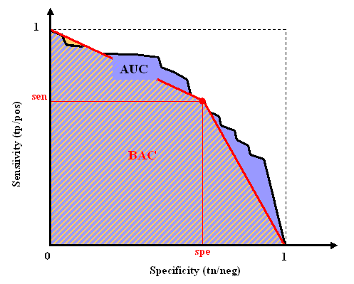
The balanced accuracy is the average of the sensitivity and the specificity, obtained by thresholding the prediction values at zero:
BAC = 0.5*(tp/(tp+fn) + tn/(tn+fp)).
The balanced error rate is its complement to one: BER = (1-BAC)
Area Under Curve (AUC)
The area under curve or AUC is defined as the area under the ROC curve. This area is
equivalent to the area under the curve obtained by plotting sensitivity against
specificity by varying a threshold on the prediction values to determine the classification
result.
The AUC is calculated using the trapezoid method. In the case when binary
scores are supplied for the classification instead of discriminant values, the curve is given by
{(0,1),(tn/(tn+fp),tp/(tp+fn)),(1,0)} and AUC = BAC.

Fscore
To provide a more direct evaluation of causal discovery, we compute various scores, which evaluate the fraction of causes, effects, spouses, and other features, which may be related to the target, in the feature set that you are using to make predictions. We will use those scores to analyze the results of the challenge. One of those, which we call Fscore, is displayed in the Result tables. The Fscore is computed in the following way:
- A set of "good" features is defined from the truth values of the causal relationships, known only to the organizers. This constitutes the "positive class" of the features. The other features belong to the "negative class".
- The features returned by the participants as a ulist or an slist are interpreted as classification results into the positive or negative class. For a ulist, all the list elements are interpreted as classified in the positive class and all other features as classified in the negative class. For an slist, the feature rank is mapped to a classification prediction value, the features ranking first being mapped to a high figure of merit. If the slist does not include all features, the missing features are all given the same lowest figure of merit.
- The Fscore is the AUC for the separation "good" vs. "not-so-good" features. It is identical to the BAC in the case of a ulist.
- The definition of "good" feature depends on the dataset and whether the test data are manipulated of not.
- For artificial and re-simulated data (for which we know the all truth values of the causal relationships), the Test data Markov Blanket (MBT) is our chosen set of "good" features. The MBT generally does NOT coincides with the Discovery data Markov Blanket (MBD) of the natural distribution, from which discovery/training data are drawn, except if the test data were drawn from the same "unmanipulated" distribution.
- For real data with probes (for which we know only the truth values of the causal relationships between target and probes), the set of "not-so-good" features is the set of probes not belonging to the Markov blanket of the target, in test data. In the case of manipulated data, since we manipulate all the probes, the set of "not-so-good" features coincides with the set of all probes. In this last case, if we define Rscore ("real score") as the score for the separation of real variable into "cause" vs. "non-cause", under some conditions, the Fscore is asymptotically linearly related to the Rscore
Fscore = (num_true_pos/num_R) Rscore + 0.5 (num_true_neg/num_R)
where num_true_pos is the (unknown) number of features in the true positive class (real variables, which are causes of the target) and, num_true_neg is the umber of other real variables, and num_R is the total number of real variables.


