|
|
LOCANET** New: result analysis ** |
How to cite the LOCANET datasets:
I. Guyon, C. Aliferis, G. Cooper, A. Elisseeff, J.-P. Pellet, P. Spirtes, and A. Statnikov.
Design and analysis of the causation and prediction challenge. In JMLR W&CP, volume 3,
pages 1-33, WCCI2008 workshop on causality, Hong Kong, June 3-4 2008.
I. Guyon, C. Aliferis, G. Cooper, A. Elisseeff, J.-P. Pellet, P. Spirtes, and A. Statnikov.
Datasets of the causation and prediction challenge. Technical Report, 2009.
Recorded presentation:
Overview of the LOCANET task (Pot-luck challenge, NIPS 2008).
Abstract:
REGED
CINA
SIDO
MARTI
in addition, the toy dataset LUCAS can be used for self evaluation. You only need to download version 0 of the datasets and use the training data to learn the causal network. The three training sets for <dataname>0, <dataname>1, and <dataname>2, are identical.
Task description:
| Provide a depth
3 causal network (oriented graph structure) around the target using
training data only, i.e., <dataname>0_train.data and <dataname>0_train.targets. |
We consider only local directed acyclic graphs. We encode the relationship as a string of up (u) and down (d) arrows, from the target.
Depth 1 relatives: parents (u) and children (d).
Depth 2 relatives: spouses (du), grand-children (dd), siblings (ud), grand-parents (uu).
Depth 3 relatives: great-grand-parents (uuu), uncles/aunts (uud), nices/nephews (udd), parents of siblings (udu), spouses of children (ddu), parents in law (duu), children of spouses (dud), great-grand-children (ddd).
Result format:
The submission should be prepared accoring to the following guidelines and emailed to: causality @ clopinet . com.
The submission format is via a text file containing the list of parents of the features of interest. The target is numbered 0. All other features are numbered with their column number in the data tables. Provide a file named: <yourlastname>_<dataname>_feat.localgraph (example Guyon_SIDO_feat.localgraph).
Example Guyon_LUCAS_feat.localgraph
0: 1 5
1: 3 4
2: 1
6: 5
8: 6 9
9: 0 11
11: 0 10
Evaluation:
A confusion matrix Cij will be computed, recording the number of relatives confused for another type of relative, among the 14 types of relatives in depth 3 networks. A cost matrix Aij, will be applied to account for the distance between relatives (computed with an edit distance as the number of substititions, insertion, or deletion to go from one string to the other, using the string description described above). The score of the solution will be computed as:
S = sumij Aij Cij
Table 1: Cost matrix (Aij):
|
Depth |
Desired |
|
1 |
1 |
2 |
2 |
2 |
2 |
3 |
3 |
3 |
3 |
3 |
3 |
3 |
3 |
X |
|
Obtained |
Relationship |
|
P |
C |
Sp |
GC |
Si |
GP |
GGP |
uud |
N |
PS |
SC |
IL |
CP |
GGC |
Other |
|
|
|
|
u |
d |
du |
dd |
ud |
uu |
uuu |
uud |
udd |
udu |
ddu |
duu |
dud |
ddd |
|
|
1 |
Parents |
u |
0 |
1 |
1 |
2 |
1 |
1 |
2 |
2 |
2 |
2 |
2 |
2 |
2 |
3 |
4 |
|
1 |
Children |
d |
1 |
0 |
1 |
1 |
1 |
2 |
3 |
2 |
2 |
2 |
2 |
2 |
2 |
2 |
4 |
|
2 |
Spouses |
du |
1 |
1 |
0 |
1 |
2 |
1 |
2 |
2 |
2 |
1 |
1 |
1 |
1 |
2 |
4 |
|
2 |
Gchildren |
dd |
2 |
1 |
1 |
0 |
1 |
2 |
3 |
2 |
1 |
2 |
1 |
2 |
1 |
1 |
4 |
|
2 |
Siblings |
ud |
1 |
1 |
2 |
1 |
0 |
1 |
2 |
1 |
1 |
1 |
2 |
2 |
1 |
2 |
4 |
|
2 |
Gparents |
uu |
1 |
2 |
1 |
2 |
1 |
0 |
1 |
1 |
2 |
1 |
2 |
1 |
2 |
3 |
4 |
|
3 |
Ggparents |
uuu |
2 |
3 |
2 |
3 |
2 |
1 |
0 |
1 |
2 |
1 |
2 |
1 |
2 |
3 |
4 |
|
3 |
Uncles/Aunts |
uud |
2 |
2 |
2 |
2 |
1 |
1 |
1 |
0 |
1 |
2 |
3 |
2 |
1 |
2 |
4 |
|
3 |
Nieces/Nephews |
udd |
2 |
2 |
2 |
1 |
1 |
2 |
2 |
1 |
0 |
1 |
2 |
3 |
2 |
1 |
4 |
|
3 |
Parents of siblings |
udu |
2 |
2 |
1 |
2 |
1 |
1 |
1 |
2 |
1 |
0 |
1 |
2 |
2 |
2 |
4 |
|
3 |
Spouses of children |
ddu |
2 |
2 |
1 |
1 |
2 |
2 |
2 |
3 |
2 |
1 |
0 |
1 |
2 |
1 |
4 |
|
3 |
Parents in law |
duu |
2 |
2 |
1 |
2 |
2 |
1 |
1 |
2 |
3 |
2 |
1 |
0 |
1 |
2 |
4 |
|
3 |
Children of spouses |
dud |
2 |
2 |
1 |
1 |
1 |
2 |
2 |
1 |
2 |
2 |
2 |
1 |
0 |
1 |
4 |
|
3 |
Ggchildren |
ddd |
3 |
2 |
2 |
1 |
2 |
3 |
3 |
2 |
1 |
2 |
1 |
2 |
1 |
0 |
4 |
|
X |
Other |
|
4 |
4 |
4 |
4 |
4 |
4 |
4 |
4 |
4 |
4 |
4 |
4 |
4 |
4 |
0 |
For artificially generated data (REGED and MARTI), the ground truth for the target local neighborhood will be determined by the generative model.
For real data with artificial "probe" variables (SIDO and CINA), we do not have ground truth for the relationships of the real variables to the target. The score will be computed on the basis of the artificial variables only.
Other task suggestions:
Using the same datasets, a number of other tasks may be performed, including:
1) Providing a graph of all causes of the target. Interested participants should use the same format as described above and return results in a file called <dataname>_feat.causalgraph.
2) Making predictions on the test sets. Intersted participants should make post-challenge submissions on the web site of the first causality challenge.
3) Learning from unmanipulated and manipulated data. Same task as 2, using training data and unlabeled test data.
4) Miscellaneous post-challenge tests.
Milestone results:
The following results were obtained at the October milestone (four participants turned in results). The Matlab score code is available as well as examples one which one can self-evaluate for LUCAS and LUCAP. The score is a value between 0 and 4, 0 being best (smallest average edit distance to the correct relationships to the target).
Table 2: milestone results
| LUCAS |
1.09 |
|
|
|
| LUCAP |
1.39 |
|
|
|
| REGED |
0.42 |
0.2 |
1.01 |
0.34 |
| SIDO |
3.44 |
3.46 |
3.25 |
|
| CINA |
2.15 |
2.23 |
2.18 |
1.74 |
| MARTI |
|
0.36 |
1.68 |
|
Preprocessed data for MARTI
Several top ranking participants of the first causality challenge have made available preprocessed data for MARTI.
FINAL RESULTS (November 19, 2008)
Table 3: final results (The scores are average distance to the true relationship in the neighborhood of the target. The scores are between 0 and 4, smaller values are better).
|
|
LUCAS |
LUCAP |
REGED |
SIDO |
CINA |
MARTI |
|
Brown |
|
|
0.27 |
3.46 |
2.23 |
0.36 |
|
De-Prado-Cumplido |
|
|
|
|
3.27 |
|
|
Dindar |
|
|
|
|
1.70 |
|
|
Engin |
|
|
|
3.48 |
|
|
|
Kirkagaclioglu |
|
|
|
|
2.16 |
|
|
Mwebaze |
0.91 |
1.80 |
0.22 |
3.46 |
2.32 |
|
|
Oguz |
|
|
|
|
1.75 |
|
|
Olsen |
|
|
0.52 |
|
3.31 |
0.21 |
|
Tillman |
|
|
0.34 |
|
1.74 |
|
|
Wang |
|
|
0.50 |
3.31 |
2.17 |
0.93 |
|
Reference A |
0.09 |
1.09 |
0.01 |
0.64 |
0.64 |
0.02 |
|
Reference B |
2.36 |
1.87 |
0.16 |
1.92 |
1.89 |
0.16 |
|
Reference C |
2.09 |
1.43 |
3.08 |
|
1.67 |
3.01 |
|
Reference D |
3.56 |
3.33 |
0.22 |
3.67 |
3.64 |
0.21 |
Reference A: Truth graph with 20% of the edges flipped at random.
Reference B: Truth graph with connections symmetrized.
Reference C: Variables in the truth graph are fully connected.
Reference D: Variables in the truth graph are all disconnected.
Result analysis:
Data generation:
Details on the datasets (not available to the participants at the time of the challenge) are available at in this report.
Fact sheets and preprints:
| Laura Brown and Ioannis
Tsamardinos |
A
Strategy for Making Predictions Under Manipulation (JMLR W&CP, 3:35-52,
2008) |
[Abstract][Fact
Sheet] |
| Catharina Olsen |
Using mutual information
to infer causal relationships |
[Fact
Sheet] |
| Robert Tillman and Joseph
Ramsey |
Fan search with Bayesian scoring
for directionality applied to the LOCANET challenge |
[Fact
Sheet] |
| Mario de-Prado-Cumplido |
Discovery of Causation
Direction by Machine Learning Techniques |
[Abstract][Poster] |
| Ernest Mwebaze,
John A. Quinn |
Fast Committee-Based Structure
Learning |
[Preprint] |
| You Zhou, Changzhang
Wang, Jianxin Yin, Zhi Geng |
Discover Local Causal Network
around a Target with a Given Depth |
[Preprint][Fact Sheet] |
Precision and recall for the probes:
In addition to the results of Table 3, we created graphs to show precision and recall for a number of subsets of probe variables:
1) parents of the target (there should be none)
2) children of the target
3) PC (parents and children), aka all depth 1 variables
4) MB -- Markov blanket (PC + spouses)
5) D2: all depth 2 variables
6) D3: all depth 3 variables
We define precision and recall as:
Precision = number_good_found / number_found
Recall = number_good_found / number_good (aka sensitivity or true positive rare)
To avoid divisions by 0, we replace 0 by a very small number both for the numerator and the denominator.
Graphs for every entrant:
A number of participants made several submissions. The last one counted towards the prizes, but we show them all in the graphs for information.
Good performance correspond to symbols found in the upper right corner (high precision and recall). In the case of CINA and SIDO, since the probes are used to assess performance and no probe is a parent of the target, several participants found 0 parents (among the probes) and have therefore a perfect precision and recall (see our conventions for the case of zero values). But other than that, very few symbols are shown in the upper right quadrant.
A large number of participants submitted only results on CINA (presumably because it has the smallest number of variables). See the analysis by dataset below for the results on CINA. Only two participants submitted results on all the datasets of the challenge: Brown and Wang. From the graphs, Wang seems to have slightly more robust results (7 symbols in the upper right quadrant for their last submission) than Brown (5 symbols in the upper right corner), but from their average score, it is the opposite (Brown's average score of 1.58 is slightly better than Wang's of 1.72). Both Brown and Wang did fairly well in this challenge.
The other participants who turned in results on more than one datasets have performances that are not as consistently good. Mwebaze has only two symbols in the upper right quadrant (for CINA) and his score on CINA is not one of the best. His good score on REGED is explained by a flaw in our metric (see the "Edit distance score" section). Olsen and Tillman have only one symbol in the upper right corner (both for CINA)
Graphs for every dataset:
The datasets LUCAS and LUCAP (toy examples) and REGEDP and MARTIP (REGED and MARTI plus probes) were not part of the challenge. See the section "probe method" below for an analysis.
We comment first on the datasets REGED and MARTI, which do not include probes.
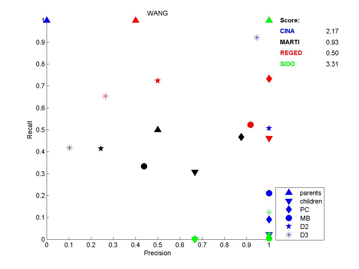
REGED: Reged is an artificial dataset (a Bayesian network trained from real microarray lung cancer data). There are 999 continous variables plus a binary target. The difficulty was that only 500 examples were available for causal discovery (similar or smaller numbers of examples are usually available for such applications). The graph of the model is very spase. This rendered our scoring method unreliable (see the "Edit distance score" section). According to our graphs, only Brown and Wang did well on this dataset. They both identified correctly the two direct causes. But Wang included three other nodes in the set of direct causes, so his precision is not so good on direct causes. However, he did also well on children PC, and MB, while Brown did not do so well on those.
MARTI: This is a modified version of REGED, on top of which a correlated noise model was added. There are 1024 continous variables plus a binary target and again only 500 examples available for causal discovery. Again only Brown and Wang did well on this dataset, although slightly worse that on REGED, which is not surprising because of the additional difficulty of filtering the noise.
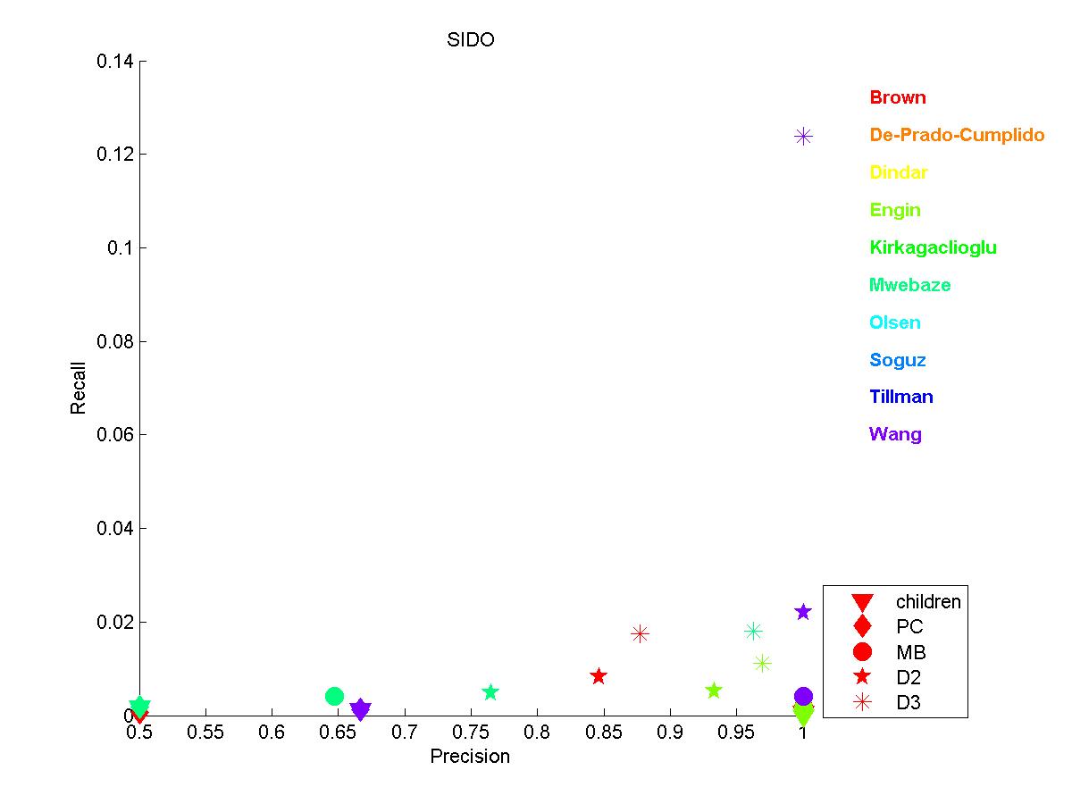
SIDO: All the participants did relatively poorly on SIDO. The recall is particularly low. See the section "probe method" below for further analysis.
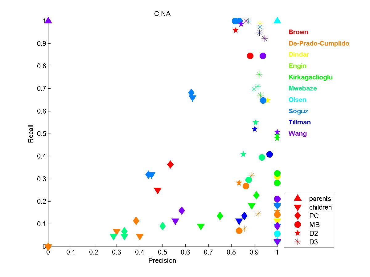
CINA: This dataset was the most popular; almost all the participants turned in results on CINA. The performances are also reasonably good, but recall is not as good as precision. See the section "probe method" below for further analysis.
Methodology:
Edit distance score:
The results of Table 3 were used to rank the participants. This score was created to globaly evaluate how well the algorithms discovered the causal structure of the data in the neighborhood of the target. We computed reference scores for comparison.
REGED:The winner turned in an empty graph. Because the graph is very spase, the empty graph obtained the best score (0.22) that could be achieved by the participants. This result reveals a flaw in our metric, which gave too much credit for correctly excluding a variable from the causal neighborhood of the target (as opposed to correctly including one). A more detailed analysis
MARTI: Similarly, the best result is obtained for the empty graph (0.21).
Probe method:
The datasets SIDO and CINA consist of real variables and artificial "probe" variables. Because we do not know the truth values of the causal relationships, the probes help us assessing how well the methods do by computing scores on the causal relationships between probes (see the report for details on probe generation). The scores in Table 3 for SIDO and CINA are computed using only the probes. The probes are features derived from the real variables and other probes using a function plus noise. Hence, no probe is a cause of the target.
Even though we made an effort to imitate the distribution of real variables when constructiong the probes, we significantly changed the graph topology, and increased the space dimensionality. Hence, the problems may have become harder that the original problems (without probes). This can be seen with our toy example LUCAS for which the original problem is a Bayesian net of known topology, which we used to emulate a "real" system. Then we added probes to that system to get the LUCAP example. We see that the score for LUCAP is worse than that of LUCAS when we flip at random 20% of the edges (reference A), while it is better for references B and C and roughly the same for reference D. These differences indicate that the probe method may not give a good indication of performance of a method on the "real" system (without probes). Further, the presence of the probes may complicate the discovery of relationships between the "real" variables.
One participant (Mwebaze) turned in results for LUCAS and LUCAP and gets slightly worse results for LUCAP than LUCAS. We also generated probe versions of REGED and MARTI, which are also artificial datasets (called REGEDP and MARTIP). This corresponds to task T5 of the post-challenge analysis of the causation and prediction challenge. Mwebaze also kindly ran his algorithms on those datasets. Scores of 3.46 and 3.49 were obtained for these datasets, very significantly worse that the scores obtained for REGED and MARTI. Hence, further work needs to go into the probe method to make it an effective tool to evaluate causal discovery performance on the real variables.
However, this does not invalidate the use of SIDO and CINA as benchmarks to test and compare causal discovery methods. We examine separately the results on SIDO and CINA:
SIDO: This dataset includes 4932 binary variables plus a binary target. There are 12678 examples, but the classes are very unbalanced (only 452 positive examples). The features are very weak predictors of the target and because of the small number of positive examples, it is very difficult to infer causal relationships. As can be seen in this figure, the precision can be relatively good, but the recall is always very poor. This means that very few of the variables that are actually in the neighborhood of the target are discovered by the algorithms, but they do not have too many false positive.
CINA: This dataset has the smallest number of variables (132) and a comparably large number of training examples (16033). This probably explains its popularity and the relatively good results obtained (see the figure). Similarly as SIDO however, recall is not as good as precision. So perhaps the tests of conditional independence are too conservative. In particular, this affects the immediate neighborhood of the target (poor recall for the parents and children, but good precision).
Qualitative analysis of CINA:
CINA is a dataset derived deom the Adult database, see details on the data preparation in our report. The predictive variables are census attributes such as age, marital status, sex, etc. The target variable is whether an individual earns more than $50K per year. A dataset derived from this same dataset and called ADA was used in the performance prediction challenge and the ALvsPK challenge.
Because of the large number of contributors to CINA in the pot-luck challenge and the good average precision of the results, we profiled all 44 true variables with respect to the frequency at which they were called parent (direct cause), child (direct effect), or whether they were found in the depth 2 or 3 layers of the netwok (regardless of relationship). We used 17 entries to make these statistics (some of which were entered by the same person).

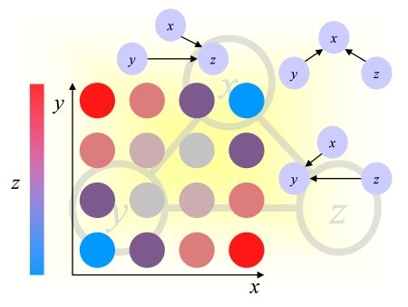
Figure 1: Profile of the real features for CINA according to the pot-luck challenge submissions.
Number of times cited in an entry as cause (black), effect (brown), layer2 (orange), layer 3 (peach).
Observations:
- All 44 features are cited at least in some entries to be within the depth 3 network.
- Because no probe is a parent of the target, the probe method is of limited use to assess whether the methods did a good job at finding parents. The precision is 0 (unless no parent is returned) and the recall is undefined (division by 0). However, the precision is usually quite good for the children and for the MB.
- Although on average the entrants has a good precision on finding children/MB/D2/D3 sets on the probes, many entrants did not include real variables as part of their parent/children/MB sets. It seems that the probes may have been too predictive. This is confirmed by looking at the set of variables most correlated to the target. The top 10 most correlated features are effects.
- The figure also indicates that the features cited as causes of the target are also very often cited as effects, and usually more often. This is surprising since the target (whether the person earns more than $50K per year) is unlikely to be a cause of most features). Among the features, which are at least called 5 times a cause or a consequence, we have the following profiles (C=number of times calles a cause; E=number of times called an effect):
age C4 E1 corr= 0.24We show in blue the variables more often called causes and in green those more ofte called effect. The age is a definite cause and this makes sense. Occupations are sometimes called causes and sometimes called effect. It is questionable whether occupation_Exec_managerial could be an effect (cited 6 times as an effect and only two times as a cause). Also very questionable is whether race_Amer_Indian_Eskimo and educationNum could be effects. On the other hand, the fact that capitalGain and capitalGain are considered effect could make sense (you can invest only if you earn a lot). Fianlly, the causal relationship of the other features (e.g. related to marital status or occupation) is not impossible.
occupation_Prof_specialty C3 E2 corr= 0.17
fnlwgt C3 E2 corr=-0.01
maritalStatus_Married_civ_spouse C3 E3 corr= 0.44
educationNum C2 E3 corr= 0.34
occupation_Other_service C3 E4 corr=-0.16
hoursPerWeek C2 E4 corr= 0.23
relationship_Unmarried C1 E4 corr=-0.14
workclass_Self_emp_not_inc C1 E4 corr= 0.02
capitalLoss C4 E7 corr= 0.14
race_Amer_Indian_Eskimo C1 E5 corr=-0.03 <--??? unrelated
maritalStatus_Divorced C1 E5 corr=-0.13
workclass_State_gov C1 E5 corr= 0.01
occupation_Exec_managerial C2 E6 corr= 0.22 <-- ?? why an effect
capitalGain C3 E8 corr= 0.22
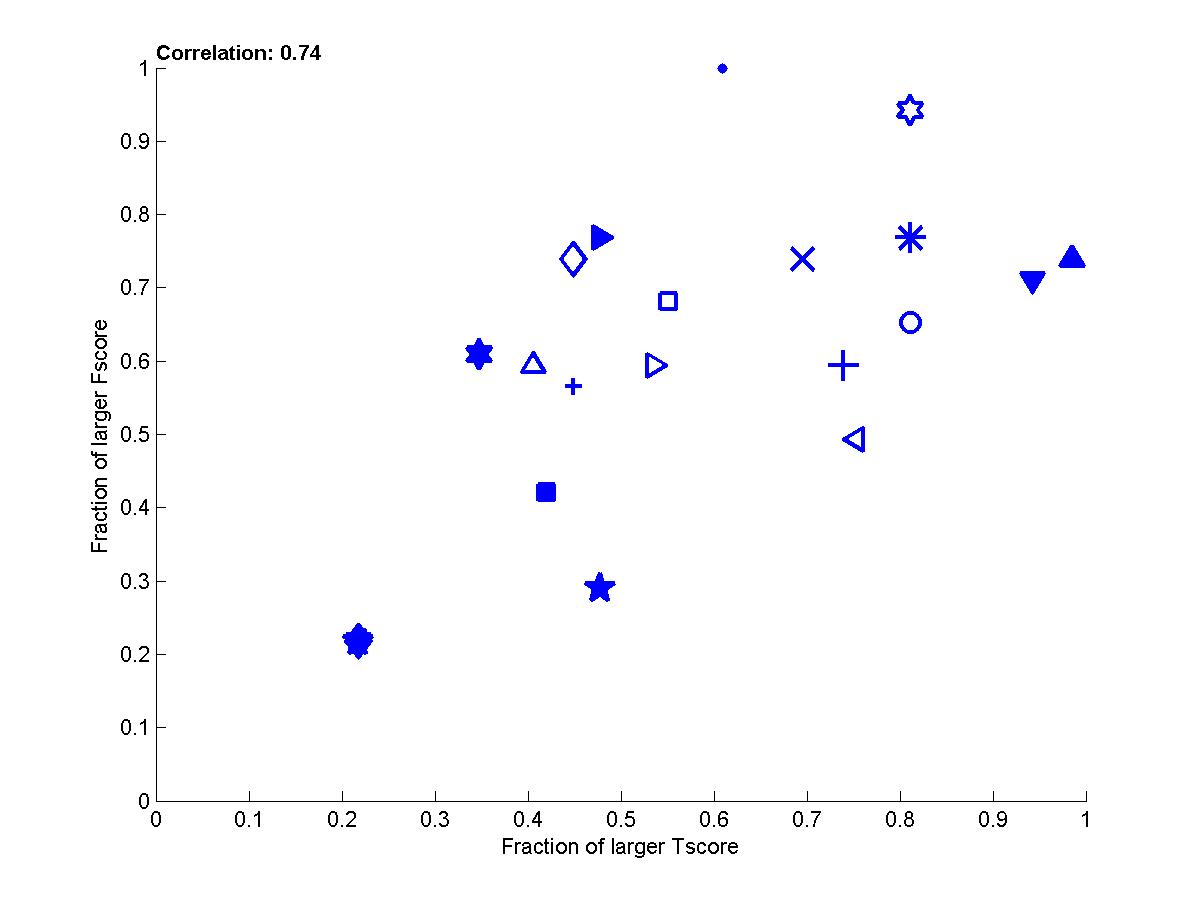
- For comparison, we investigated which features are selected by univariate methods. The top 15 real features selected by Marc Boullé (winner of the causation and prediction challenge for CINA, see the full triangle pointing up in this graph) coincide with the 15 features most correlated to the target according to the Pearson correlation coefficient (although not exactly in the same order):
maritalStatus_Married_civ_spouseThe majority of these highlly correlated features are found in the top half of the features preferred by the pot-luck challenge participants (outlined in red). Three (educationNum, marital_staus_Never_married, and sex) are tie with the feature just in the middle (outlined in orange) -- educationNum is cited 5 times as a direct cause or effect. The feature outline in black is just below the features with median score. So, overall, it is fair to say that correlation plays an important role in the selection of features, which are in the neighborhood if the target.
relationship_Husband
educationNum
maritalStatus_Never_married
age
hoursPerWeek
relationship_Own_child
capitalGain
sex
occupation_Exec_managerial
relationship_Not_in_family
occupation_Prof_specialty
occupation_Other_service
capitalLoss
relationship_Unmarried
The fact that sex and educationNum rank lower according to the participants could be explained by the fact that they are independent of the target conditionned on other variables (more direct effects).
We thought it would be interesting to compare the predictive power of feature sets. We made a small comparison of predictive performance by training on real features and testing on the test set (for CINA 0). We ranked the features is several ways: according to the Pearson correlation coefficient, according to Gram-Schmidt orthogonalization (GS) that is a forward selection method looking for complementary features, and according to the ranking of Figure 1. We preprocessed data by feature standardization and trained a linear ridge regression classifier. To make is a fair comparison, the feature selection algorithms we run in the same conditions as those of the challenge, on the 132 variables (including the probes), then the probes were removed. The results are shown in Figure 2.
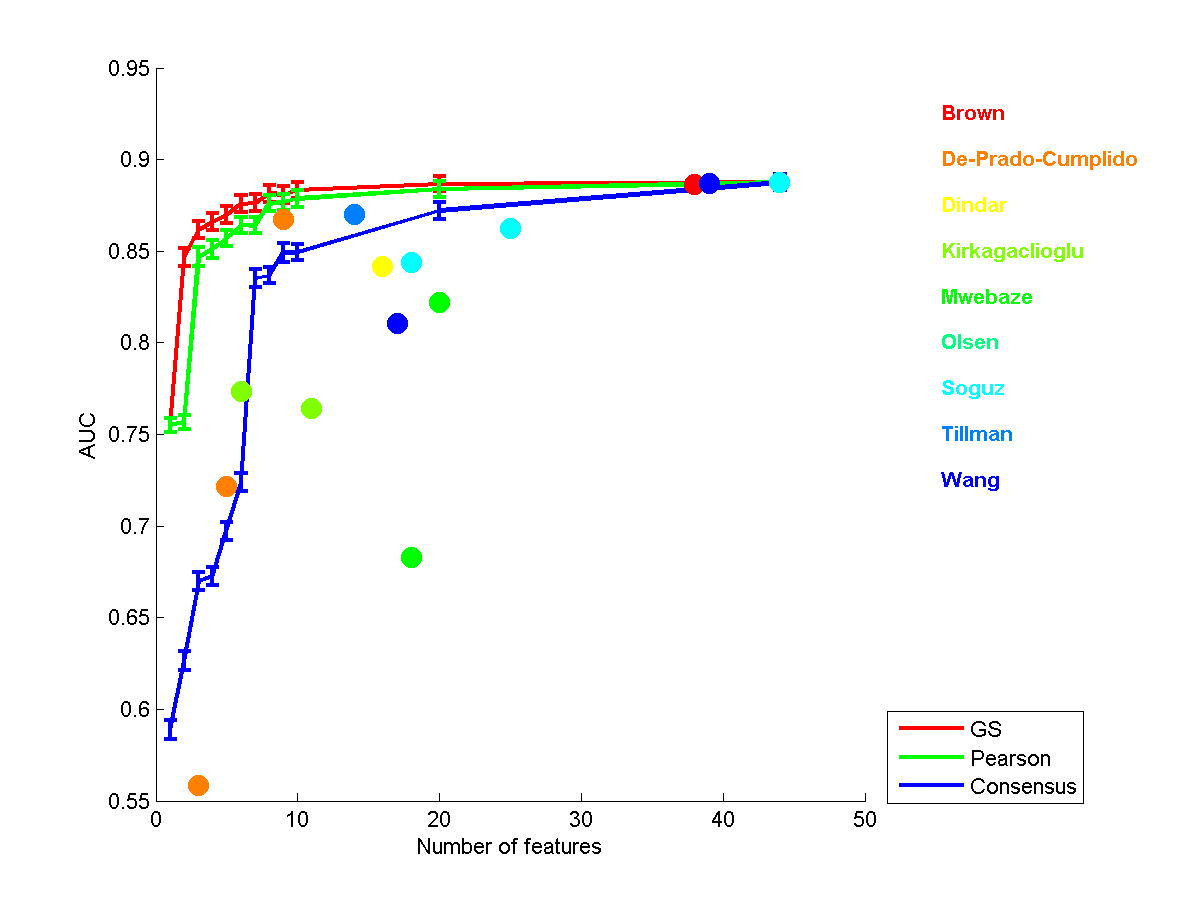
Figure 2: Performances on test data as a function of the number of features. Consensus refers to the ranking from Figure 1.
As can be seen, the best results are obtained by training on all features. GS allows getting more compact sets of features, but it is closely followed by Pearson. The Consensus method does not perform very well. It may be argued that the ranking of Figure 1 does not yield consistent complementary feature subsets. For comparison, we also show the performances obtained using the Markov blanket (MB) of the target (parents, children, and spouses) for all the entries of the participants. Also, the best entry in the causation and prediction challenge by someone who used a causal discovery algorithm for feature selection (Jianxin Yin) has AUC=0.83 with 11 features (not shown on the figure). Examining Figure 2 reveals that the performances of the challenge participants using MB features are still always lower than for GS and Pearson.
Correlation does not allow us to get the most compact feature sets. However, as we have pointed out in our analysis of the causation and prediction challenge, the Markov blanket empirically determined from a finite training set is not necessarily the best feature set (neither most predictive nor most compact). It is instructive to examine the top ranking features selected by Gram-Schmidt orthogonalization:
Features outside the MB may be very predictive if they are hubs (like educatioNun and age). The top ranking features from Figure 1 include capitalGain, capitalLoss occupation_Exec_managerial, and maritalStatus_Married_civ_spouse, but not educationNum and age. From the point of view of causal discovery, the two variables educationNum and age may be indirectly related to the target. For instance educationNum and age may be a cause of "occupation". Since there are many possible occupations, the information is diluted among several variables, some of which may not be found significantly related to the target by the algorithms.maritalStatus_Married_civ_spouse
educationNum
capitalGain
occupation_Exec_managerial
capitalLoss
age
Conclusion:
The results on CINA, in light of the semantics of the features are mixed:
If we believe the results of the participants, "age" is one of the determining factors that affects earnings (that makes sense) and if you earn a lot of money, you are likely to earn or loose a lot by investing it (that makes sense too). You are also more likely to get (and remain) married, but you will be putting a lot of hours per week. As a consolation, your comfortable earnings will push your carrier and you will become a manager, unless you decide to retire in the North and become an Eskimo (I don't think so)!
It is unclear whether using the tools of causal discovery brought us a lot more information that simple correlation would have:
- most features cited as cause or effect of the target rank among the most correlated features
- there is usually no consensus on the causal diirection among the participants
- when there is a large consensus on the causal direction, the result is sometimes suspicious given the semantics of the feature
- a simple ranking in order of correlation yields nested feature subsets always more predictive than the Markov blanket.